

As my adios to the West Village newsletter, I thought it appropriate to not only drop a little spreadsheet knowledge on you… but also to leave you with the holy grail of West Village delivery and takeout restaurants wrapped up into a naughty little spreadsheet burrito. It also notes where these places have corresponding locations elsewhere in Manhattan and Brooklyn (in case you are planning on skipping town like us). Your welcome!!
One thing I would like to caveat with these delish establishments, is that I do NOT take responsibility for any changes in restaurant sanitation grades. As we all have come to know, these seem to fluctuate daily… so you are on your own in terms of monitoring when yesterday’s “A” becomes tomorrow’s “Grade Pending.” You can do that here.
Our lesson du jour (other than how to be lazy and NOT make dinner) involves using Filters, which can be super key in sifting through data quickly.
To access our quick Filtering how-to’s, please check out our most recent blog posts (available for Mac 2011 below and PC 2007/2010 click here).
USING FILTERS
Many spreadsheeters sort their data and then scroll up and down their page to a view a specific tranche of data. Filtering allows you to sift through your data based on certain criteria.
1. Download the sample file (Filters) that is used in the lesson: visit the Tips & Tricks page of www.ExcelRainMan.com.
2. Ways to add filters to your data:
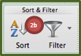
a. Standard Toolbar, select Filter


b. Data tab, Sort & Filter group, click Filter

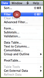
c. Data menu, select Filter

d. Highlight the header row, then use the Keyboard Shortcut: Command – Shift – F
3. Notice the arrows in the bottom right corners of the header row (in this case Row 1)
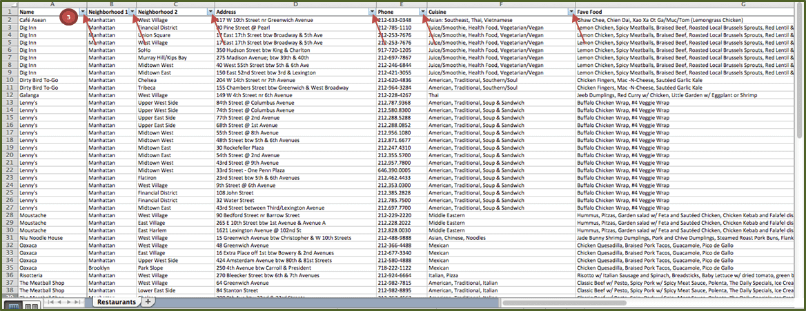

By clicking on the bottom right arrow, of any of the column headers, you will see a list of all of the individual cell contents in the column. You can then select the contents you want to view by simply checking on the pertinent boxes.
This is a very useful feature in sifting through data in Excel. Some general tips:
• If you want to view most of the items, you may want to uncheck the boxes of the items that you do not want to see.
• If you want to view a few of the items, you may want to uncheck the Select All box, and then check items that you want filter.
4. To see which restaurants deliver to the West Village, select the Neighborhood 2 filter (arrow) in cell C1.
5. Uncheck Select All
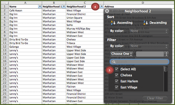

6. Scroll down and select West Village, then just click outside of the Filter dialog box (and your selected criteria is filtered upon)
7. Result is the rows with the criteria selected in column C (West Village)
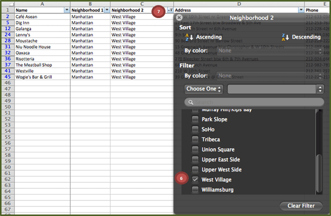

Please note that when you filter the data, the rows are still there. You are just zooming in on the specified filtering criteria. Notice how the row numbers 2, 5, 12, 24, … on the left are in blue and the remaining row numbers (1, 46…) are in black. This signifies that there are hidden rows in the data set due to the filter used.
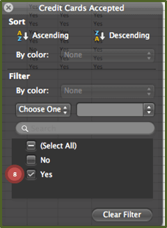
8. Now that we have the restaurants that deliver in the West Village delivery radius, we realize that we must pay with credit card as there is not much is our wallet. Scroll to the right and filter on the Credit Cards Accepted column (J). This time make sure Yes is selected.

9. Finally, while these legs could use some walkin’, if you are feeling a little lazy, go to the Delivery column (H) and be sure to select Yes (really unselect No).
10. Last but certainly not least, read through the Cuisine column (F) and our Fave Food column (G) to figure out what you want to nosh on. Bon Appetit!
REMOVING FILTERS
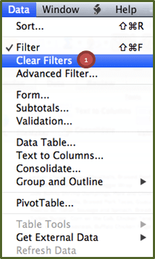
1. To remove the Filter selections made and bring all of the data back to the screen, go to the Data menu, select Clear Filters

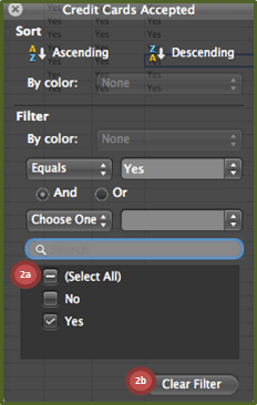
2. To remove the Filter selections for each individual column, you must go to each column (select any cell in the column) and do one of the following:
a. Click on the Arrow of the columns that you filtered (notice the funnel next to the arrow). Check the Select All box.
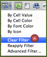
b. Click on the Arrow of the columns that you filtered, select Clear Filter.

c. Standard Toolbar, select the Filter dropdown, select Clear Filter

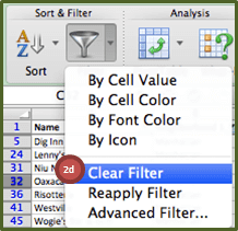
d. Data tab, Sort & Filter group, click Clear Filter

3. To remove the Filters entirely (and bring all of the data back to the screen), do one of the following:
a. Standard Toolbar, unselect Filter
b. Data tab, Sort & Filter group, unselect Filter
c. Data menu, unselect Filter
d. Keyboard Shortcut: Command – Shift – F
In case you want to dive into Filters more and some other topics, for the month of June Video Tutorial 1 – Getting Started is FREE! This includes Navigating the Ribbon, Freezing and Unfreezing Panes, Sorting, Creating Filters and Using Paste Special features.
Also, use the code Delivery20 to receive 20% off any purchase of Video Tutorials.
The discount and FREE VTs apply for the PC 2010/2007 and Mac 2008 versions of Excel as well. Mac 2011 and PC 2013 tutorials are coming soon… Stay tuned!