Remember back in the day when the PC 2007/Mac 2008 versions of Excel came out and everyone freaked? Email after email flooded the Excel Rain Man inboxes with all kinds of questions… “Where is the file menu?!?” “What is up with this Ribbon!?!” “Why are Pivot Tables under the insert tab?!”

Well we all have come a long way baby…
– PC 2003/Mac 2004 is now vintage
– PC 2007/Mac 2008 has grown on us
– PC 2010/Mac 2011 is ballin’ out of control

Just one of the reasons that the latest version of Excel is rocking everyone’s world is the new Sparklines feature!

Sparklines are a nice visual to add next to any data set to show trends within the data including low points and high points to help draw your eye to them.

The 3 types of sparklines you can use are Line, Column and Win/Loss.

So if you want to amp up your reports or just amend the way you view and present your data… See our latest blog post on how to assemble Line Sparklines (Mac 2011 below or PC 2010 click here)… this example may just help you decide which receiver to pick in Round 1 of your fantasy draft!

CREATING SPARKLINES
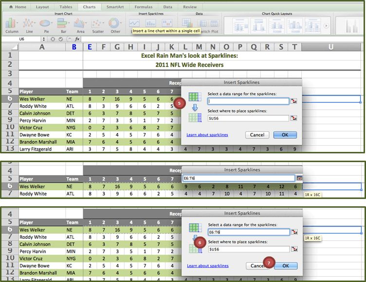
1. Place the cursor in cell U6
2. Go to the Charts tab, Insert Sparklines group
3. Select the type of sparkline you want to create:

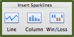
4. In this example, we will work with Line sparklines, so select Line

The Insert Sparklines dialog box appears:
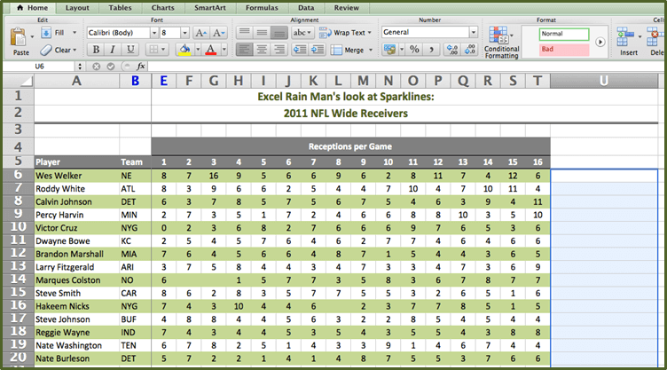
5. Select Data Range for the 1st sparkline
In this case we will select Wes Welker’s receptions for Games 1 – 16 which are in cells E6:T6

6. Place (has cell U$6$) is already populated because this is where we placed the cursor in step 1
You can change the location of the sparkline here, but we suggest having it next to the data for its full effect

7. Select OK

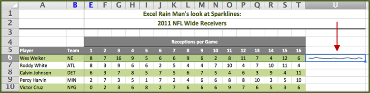
Notice the sparkline that now appears in cell U6

CUSTOMIZING SPARKLINES (make ‘em pop!)
Before we copy and paste our sparklines for all top wide receivers, we might as well make them look good!
1. Again, place the cursor in cell U6 (where the sparkline is)

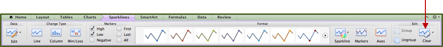
2. Go to the Sparklines tab, Format group

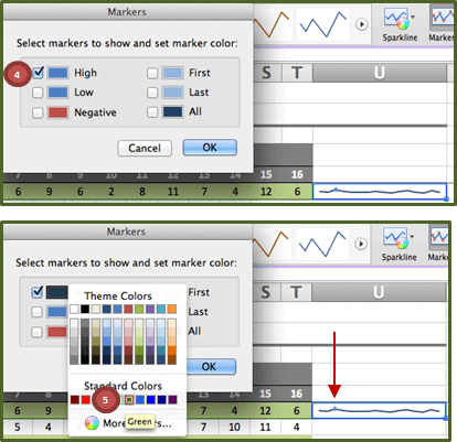
3. Select Markers

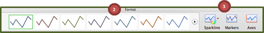
4. Check High Point, then select the blue rectangle next to it to change the color

5. Let’s select Green to signify which game each wide receiver had the most receptions

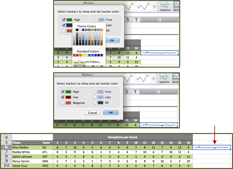
6. This time check Low, then select the rectangle next to it to change the color

7. Let’s select Dark Red to signify which game the wide receiver had the fewest receptions

8. Select OK

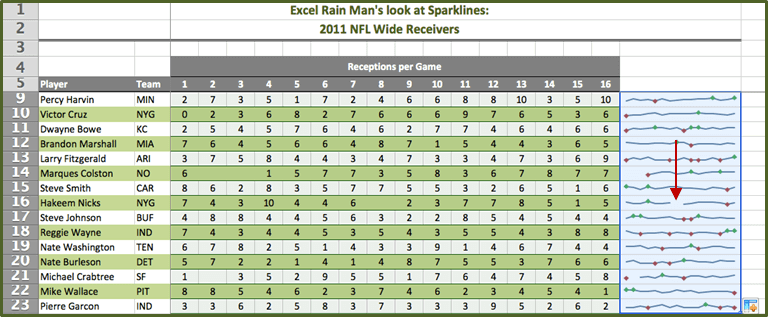
9. Finally, you can drag or copy/paste the custom sparkline you created in cell U6 to the remaining cells in column U

10. Notice how in the weeks where a wide receiver did not play (meaning receptions for that game are blank) there is a break in that sparkline
For example: Hakeem Nicks was inactive for game 8 (Giants vs. Patriots – week 9) of the 2011 NFL season. Therefore the low point on his sparkline is when he had 1 reception in game 15 as opposed to when he was inactive for game 8.

REMOVING SPARKLINES
1. Simply highlight the sparklines you want to remove

2. Right click, select Sparklines, and select Clear Selected Sparklines

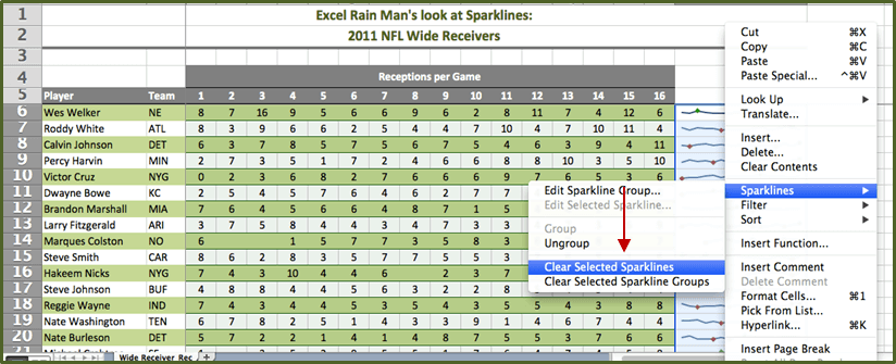
OR go to the Sparklines tab, Edit group, select Clear

Voila your sparklines are gone…

Have your spreadsheets lost their spark? Contact Excel Rain Man and we will teach you how to spice it up!